Unsupervised Learning | Python Implementation

In the previous blog, we learned about the supervised learning algorithms and how to implement them using Python, now we will discover about the unsupervised learning algorithms and how to implement them using Python. So, let us begin with this image which shows how unsupervised learning is different from supervised learning.

Supervised vs Unsupervised Learning

Look at the left part of the image, here the teacher is teaching Joe, which is the case of supervised learning i.e model learns through labeled data. While in the right part of the image Joe is learning on his own, which is the case of unsupervised learning i.e model learns through unlabeled data.

What is Unsupervised Learning?

Unsupervised learning refers to a set of machine learning algorithms/methods that discover patterns in given input data that is neither labeled nor classified which means they analyze and cluster unlabeled datasets.

Unsupervised Learning Example

Some of the common examples of unsupervised learning are - Customer segmentation, recommendation systems, anomaly detection, and reducing the complexity of a problem.

Types of Unsupervised Learning Algorithm

The two major types of unsupervised learning are:

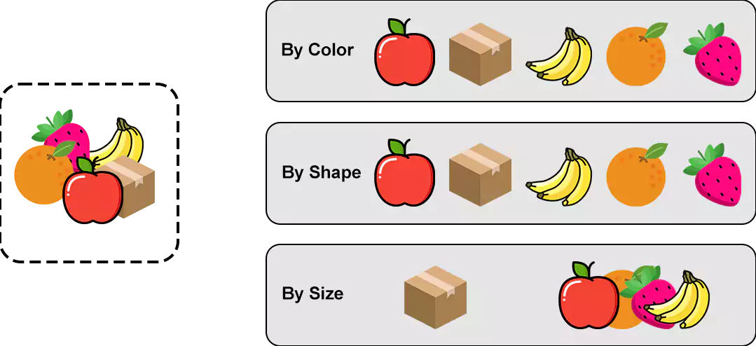
Clustering 

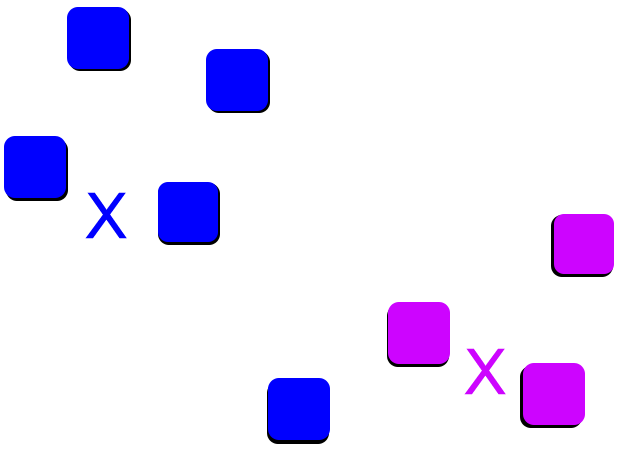
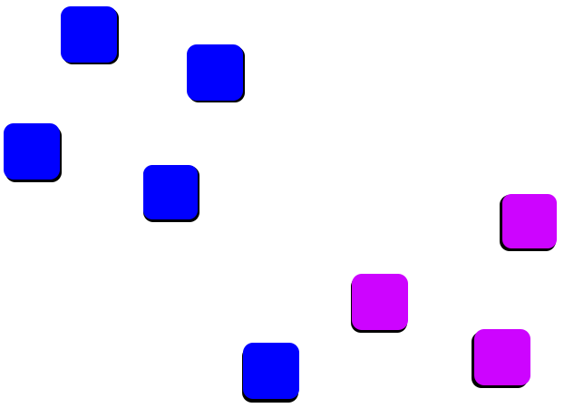
The division of given data points/examples into X number of groups called a cluster, such that datapoints/examples of each group are similar and dissimilar from the data points of other groups. Look at the image below to get an idea of how clustering works.

Properties of Clusters

1. All data points in a cluster should be similar to each other, which means the distance between the data points should be as minimum as possible.
2. The data points of different clusters should be as different as possible, which means the clusters should be far away from each other.

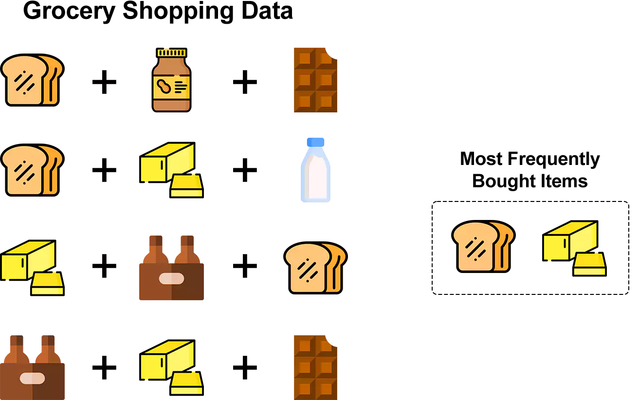
Association Analysis

It is a process to discover how data points/items in a dataset are associated with each other. It is mostly used for Market Basket Analysis i.e which items are bought together, say if someone buys bread so he may buy butter, jam, peanut butter, or any other spread that's why these items are placed together in a grocery store. Take a look at the image below.

Why we need Unsupervised Learning?

• It finds all hidden and complex patterns in data.
• It is closer to real AI, as the learning fashion of an unsupervised learning model is the same as a human being.
• We don't have input data and corresponding output in the real world, which makes unsupervised learning very useful.
• Very helpful in exploratory analysis.

Tools we are going to use

• Python3.9 Download Link

• Jupyter Notebook Download Link

• Scikit Learn Download Link

• NumPy Download Link

Common Unsupervised Learning Algorithms

• K-means Clustering
• Hierarchical Clustering
• DBSCAN
• Apriori
• FP-Growth

K-means Clustering

K-means is a popular clustering algorithm. It is a distance-based, iterative clustering algorithm where the distance between the data point and the centroid of the cluster is measured in order to assign a data point to a particular cluster. The goal of this algorithm is to minimize the sum of distances between the data points and their corresponding cluster centroids.

How does K-means work?

Below are the steps to describe the working of K-means.

Step1: Decide the value of K i.e picking the number of clusters.

Step2: Select n number of random data points from the dataset as the centroid; here, n = K.

Step3: Allot the data points to the nearest cluster centroid.

Step4: After assigning each data point to a particular cluster, recalculate the centroid.

Step5: Redo steps 3 and 4 till the maximum number of iterations are reached(set by you).

Read me before moving to the coding section

• The below code is just a demonstration of how to apply scikit-learn and other libraries.
• Random training data is used.
• Limited use of parameters in these code snippets.
• And these points apply to all code snippets you will see in this article/post.

Python Implementation

#import necessary libraries
from sklearn.cluster import KMeans
import numpy as np

#Create random data
X = np.array([[1, 2], [1, 4], [1, 0],
              [10, 2], [10, 4], [10, 0]])
#Create model
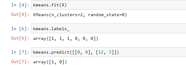
kmeans = KMeans(n_clusters=2, random_state=0)

#Feed data to model
kmeans.fit(X)

#Predict the output for X
kmeans.labels_

#Predict output for unseen data
kmeans.predict([[0, 0], [12, 3]])

Output

Hierarchical Clustering

It is a simple method that seeks to build a hierarchy of clusters. 

Hierarchical clustering has two main types:

1. Agglomerative hierarchical clustering 
2. Divisive Hierarchical clustering

Agglomerative hierarchical clustering is commonly used in industry and in this post we will briefly discuss it. So, let's begin.

The main objective of this algorithm is to merge clusters at each iteration until we are left with a single cluster. As this technique merges the clusters, so it is also known as additive hierarchical clustering.

How does Agglomerative hierarchical clustering works?

Below are the steps to describe the working of Agglomerative hierarchical clustering.

Step1: Determine Proximity matrix; proximity matrix is just a square matrix that stores the distances between the clusters.

Step2: Each data point is considered as an independent cluster.

Step3: Combine the 2 nearest clusters and update the proximity matrix.

Step4: Repeat Step3 until a single cluster is left.

Look at the picture below to get a more clear idea.

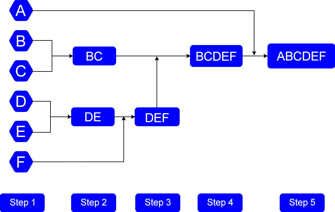
To visualize agglomerative hierarchical clustering we use Dendrogram, which is a tree-like structure that stores the sequence of events(merges). Take a look at the images below and observe the change of color.

 Python Implementation

#import necessary libraries
from sklearn.cluster import AgglomerativeClustering
import numpy as np

#Create random data
X = np.array([[1, 2], [1, 4], [1, 0],
              [10, 2], [10, 4], [10, 0]])
#Create model
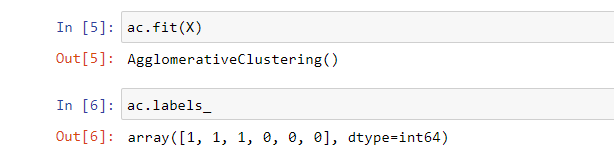
ac = AgglomerativeClustering()

#Feed data to model
ac.fit(X)

#Predict the output for X
ac.labels_

Output

On the other hand, divisive hierarchical clustering is just the opposite of agglomerative hierarchical clustering. In case of divisive, we start with a single cluster and separate it into clusters on each iteration. This approach is not used that much in the industry.

DBSCAN

DBSCAN stands for Density-based spatial clustering of applications with noise. This algorithm works by recognizing data points in a crowded region of feature space, where data points are not well spaced i.e less gap between data points.

Why we need DBSCAN?

Now, the important question is why we need this algorithm? When we are having algorithms like K-means, hierarchical clustering does the job very well. Below are a few points to understand the need of DBSCAN:

1. DBSCAN is more accurate than K-means and hierarchical clustering when dealing with data containing noise i.e fuzzy data.
2. It can accommodate large datasets.
3. We don't need to define the number of clusters.

DBSCAN Parameters

This algorithm requires only 2 parameters. 

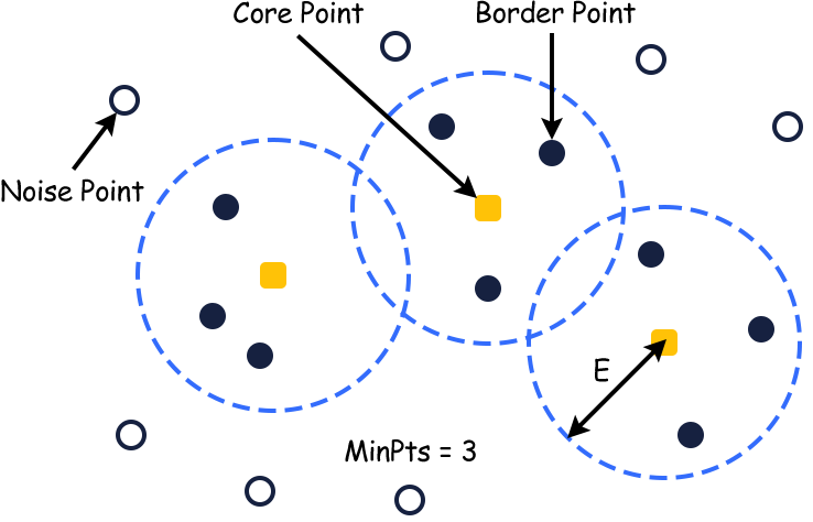
1. eps(Epsilon): It is a criterion for considering a point neighbor or not for a particular data point. If the distance between two data points is less than or equal to the value of eps, then they are considered neighbors. For larger values of eps, a large number of data points including noise will be in the same cluster. On the other hand for smaller values of eps, a large number of data points are considered as noise which is also not good. For finding the optimal value of eps we use the k-distance graph.
2. minPoints(n): In order to consider a spatial region as dense, we require a minimum number of points 'n' to cluster together. Its value depends upon the size of the data set, for a large dataset 'n' should be large too and vice-versa.

Take a look at the figure below.

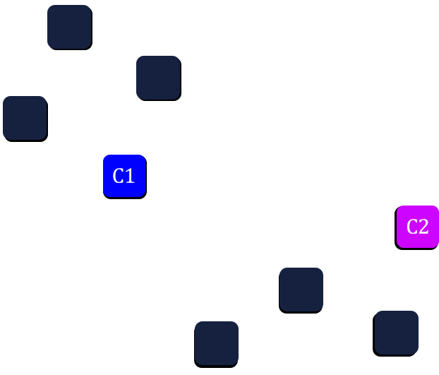
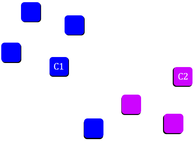
Working of DBSCAN

Below are the steps to describe the working of DBSCAN.

Step1: Randomly pick point 'p'  from the dataset and assigned it as cluster 1. 

Step2: Count the number of points 'z' located within the eps distance from p. If z is greater than or equal to minPoints(n), then p will be considered as a core point and all the eps-neighbors will be a part of cluster 1.

Step3: Then, it will find the eps-neighbor of each data point in cluster 1 and expand cluster 1 by adding those points. 

Step4: Once cluster 1 has no more data points to fill in, another unseen random data point will be picked from the dataset and assigned as cluster 2.

Step5: It will repeat the same steps for cluster 2 but will not consider those points that are already a part of cluster 1.

Step6: N number of clusters will be created in the same manner till all data points are not clustered.

Python Implementation

#import necessary libraries
from sklearn.cluster import DBSCAN
import numpy as np

#Create random data
X = np.array([[1, 2], [2, 2], [2, 3],
             [8, 7], [8, 8], [25, 80]])
#Create model
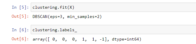
clustering = DBSCAN(eps=3, min_samples=2)

#Feed data to model
clustering.fit(X)

#Predict the output for X
clustering.labels_

Output

Apriori Algorithm

(I encourage you to study association rule learning before moving to this section.)

Apriori belongs to the association analysis class. This algorithm uses association rules to find out how strong or weakly two objects are connected to each other. The key idea behind this algorithm is that it uses prior knowledge of frequent itemset property which is a subset of a frequent itemset that must also be a frequent itemset. 

A frequent itemset is the set of items that occurs more frequently in comparison to other items. Example: Consider two transaction, X =a {1,5,7,9} and Y ={4,6,7,9,13} here 7,9 are frequent itemsets.

Factors on which this algorithm depends are: support, confidence, and lift. 

• Support: It tells us about the popularity of a particular item. For an item X, it is defined as the ratio of the number of transactions containing X to the total number of transactions. 
• Confidence: It shows how likely Y is purchased when X is purchased. It is defined for 2 items that occur together. It is the ratio of the number of transactions containing both X and Y to the total number of transactions. 
• Lift: It is the ratio of confidence to support.

Apriori Working

Below are the steps to describe the working of Apriori.

Step1: Set values of minimum support and confidence and k.

Below is the transaction table.

Transaction Database

Transaction ID	Items
T1	A
T2	X, B, A, U
T3	R, U, B
T4	U, A, B
T5	U, X, G

minimum support = 2, minimum confidence = 75% and k =2

Step2(k=1): Generate a  table containing the support count of each item present in the database and sort it in descending order, this table is called candidate set.

Candidate Set(k=1)

Item Set	Support Count
U	4
A	3
X	3
B	3
R	2
G	1

Step3: Now, remove the items from the candidate set whose support count is less than min support count. Update the candidate set.

Updated Candidate Set(k=1)

Item Set	Support Count
U	4
A	3
X	3
B	3
R	2

Step4(k=2): Form association rules and generate another candidate set(2). Remove those associations whose support count is less than the minimum support count and update the table.

Candidate Set(k=2)

Associations	Support Count
{A, X}	2
{A, R}	1
{X, B}	1
{X, U}	2
{B, A}	2
{B, U}	3
{A, U}	2
{R, U}	1

                                                                                      

Updated Candidate Set(k=2)

Associations	Support Count
{A, X}	2
{X, U}	2
{B, A}	2
{B, U}	3
{A, U}	2

Step5: Calculate the confidence for each association and put it in another table. Remove those associations whose confidence is less than the minimum confidence value. Update the confidence table.

Association Table

Associations	Confidence
{A, X}	66.6%
{X, U}	66.6%
{B, A}	66.6%
{B, U}	100%
{A, U}	66.6%

 

Final Association Table

Associations	Confidence
{B, U}	100%

Step6: Calculate the lift value for the final associations. If the lift value is equal to one it means there is no association, if it is less than 1 there is very little association and if it is greater than 1 there is high association; association means chances of items being bought together.

FP-Growth

(I encourage you to study FP-Tree before moving to this section.)

FP-Growth is an upgrade of Apriori. This algorithm permits frequent itemset determination without candidate itemset generation.

Why we need FP-Growth?

In the case of Apriori, a new candidate set have to be constructed at each step which requires repeated scanning of the transaction database. Due tho which apriori algorithm becomes slow. FP-Growth is a solution for this problem as there is no candidate set generation required which makes FP-Growth less time taking than Apriori.

FP-Growth Working

Below are the steps to describe the working of FP-Growth.

Step1: Set minimum support, determine the support count of each item in the transaction database, and set the priority value depending upon the support count.

Below is the transaction database.

Transaction Database

Transaction ID	Items
1	E,A,D,B
2	D,A,C,E,B
3	C,A,B,E
4	B,A,D
5	D
6	D, B
7	A,D,E
8	B, C

minimum support =3

Priority Table

Transaction ID	Items	Ordered Items
A	5	3
B	6	1
C	3	5
D	6	2
E	4	4

 

Step2: Order the items according to priority.

Ordered Table

Transaction ID	Items	Ordered Items
1	E,A,D,B	B,D,A,E
2	D,A,C,E,B	B,D,A,E,C
3	C,A,B,E	B.A.E.C
4	B,A,D	B,D,A
5	D	D
6	D, B	B, D
7	A,D,E	D,A,E
8	B, C	B, C

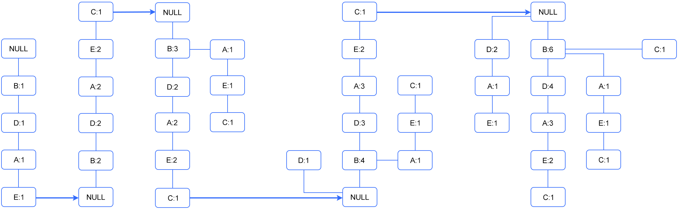
Step3: Draw FP-Tree. 

1. If it is a unique transaction form a new path and set the counter for each node to 1. 
2. If it shares a common prefix itemset then increment the common itemset node counters and create new nodes if needed.

Below is the complete FP-Tree for this transaction table consisting of 5 steps.

Suggestion

I encourage you all to read scikit-learn documentation. Also, study these algorithms and techniques: PCA(principal component analysis), Gaussian mixture models, independent component analysis, and dimensionality reduction.

Conclusion

This article learned about the common unsupervised learning algorithms and how to implement them in Python. These are the most commonly used algorithms to deal with unlabeled data. Still, there are many other algorithms know to us and applying a particular algorithm completely depends upon the problem. Also, we have not implemented  Apriori and FP-Growth in this article, as we need real data to apply these algorithms and before that, we need to understand how to prepare real data for training a model which we will be studying in the upcoming tutorial.

I hope, you got an idea of supervised learning algorithms and their implementation. Still, if you have any questions leave your comment and I will be there to help you. 

Related Blogs

• Supervised Learning with Python Implementation
• What is Machine Learning | How Python is used with Machine Learning
• What is Graph in Data Structures? | Techofide
• Data Structures with Python

Also, Read

• How to Become an Ethical Hacker | Techofide
• How To Install Arch Linux [Installation Guide] 2023 | Techofide