Supervised Learning | Python Implementation

In this blog, we will acquire knowledge of supervised learning algorithms and how to implement them using Python. So, let us start with a quote from the machine learning genius. 

"No one knows what the right algorithm is, but it gives us hope that if we can discover some crude approximation of whatever this algorithm is and implement it on a computer, that can help us make a lot of progress." ~Andrew Ng

For a quick recap about Machine Learning, take a look at this article What is Machine Learning | How Python is used with Machine Learning

What is Supervised Learning?

Supervised learning refers to systems and algorithms that teach a model by feeding input data and correct output data/labels. Supervised learning is mostly used to create machine learning models for two types of problems.

Regression: 

Regression tasks are specified by labelled datasets that have a real value(numeric). Examples: Predicting house price, predicting bitcoin future price, regression analysis in business, and many more.

Classification:

The final prediction of the model will be a class(cats or dogs, human or plant). Examples: Classifying email as spam or not, determining whether or not x will be a defaulter of the loan, Predicting the chances of any disease.

How Supervised Learning is Different from Unsupervised Learning?

In the case of unsupervised learning, the model is trained using unlabeled data and is let on to act on the unlabeled data without any supervision i.e the model learns from the inputs only but in supervised learning, the model is trained using labelled data i.e inputs and outputs both are provided. While supervised learning is used to solve regression and classification problems, unsupervised learning is used to solve clustering, association, and dimensionality reduction problems.

Till this point, we have got a basic idea of different machine learning algorithms/approaches to solve different kinds of problems. Now, let's take a deep dive into supervised learning algorithms.

Tools we are going to use

• Python3.9 Download Link

• Jupyter Notebook Download Link

• Scikit Learn Download Link

• NumPy Download Link

Common Supervised Learning Algorithms

• Linear Regression

• Logistic Regression

• Support Vector Machines(SVM)

• K-Nearest Neighbors(KNN)

• Naive Bayes Classifier

• Decision Trees

Linear Regression

It is one of the best statistical methods that study the relationships between the dependent variable(Y) with a given set of independent variables(X_i). The relationship can be established with the help of fitting the best line; y = ax + b​(called the slope-intercept form of the equation of a line). Below is the picture of such a line.     

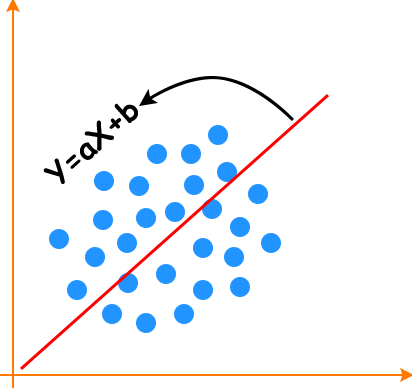
Simple Model

Output            ~   Real number

Hypothesis    ~    y(estimate) = w1x1 + w1x2 + ... + wnxn + b ; where 'w' is  assigned weight and 'b' is bias

Read me before moving to the coding section:

• The below code is just a demonstration of how to apply scikit-learn and other libraries.
• Model is trained using random samples of data.
• Here .score() is used only for training accuracy.
• Limited use of parameter in these code snippets.
• And these points apply to all code snippets you will see in this article/post.

Python Implementation:

#import required libraries
import numpy
from sklearn.linear_model import LinearRegression

#create input data
X = numpy..array([[0,5],[3,7],[8,4]])
Y = numpy.dot(X, np.array([3,2])) + 7

#create Model
reg = LinearRegression()

#Supply data to model
reg.fit(X,Y)

#check training score
reg.score(X,Y)

#Predict Output for some other data
reg.predict(numpy.array([[3,5],[4,7]))

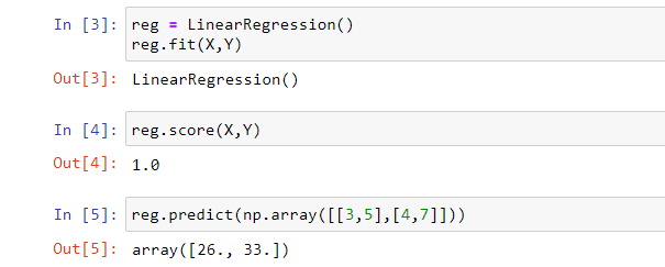
Output:

• Here reg.fit is used to build a linear regression model.

• reg.score is used for training accuracy, in case of model accuracy .score() calculates the score for the estimation/prediction value. 

Logistic Regression

Logistic regression is used to estimate discrete values(0 or 1) on a given set of independent variables. The name of this algorithm is derived from the function which is the core of the method i.e logistic function/sigmoid function.

Mathematical equation: σ(z) = 1/1 + e-z ; σ/sigma represents sigmoid function;

z = w1x1 + w1x2 + ... + wnxn + b ; z is sum of input features multiplied with the weight 'w' ,and bias 'b'.

For z = very large value(+ infinity)  : Output will be 1 and for z = very small value(- infinity) : Output will be 0.

The final output will be y(estimate) = σ(z)   Take a look at the fig. below.

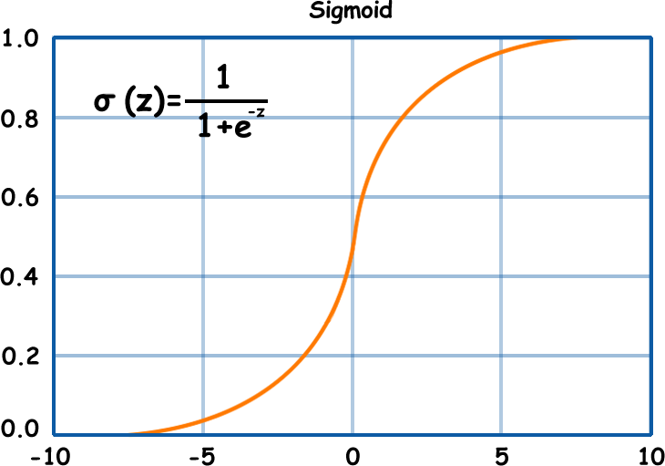
Simple Model          

Output            ~   0 or 1

Hypothesis    ~   z =  w1x1 + w1x2 + ... + wnxn                                       

Python Implementation: 

#import required libraries
from sklearn import datasets 
from sklearn.datasets import load_iris
from sklearn.linear_model import LogisticRegression

#Here we are using Iris dataset which scikit learn provides
X,y = load_iris(return_X_y =True)

#Create Model
lgr = LogisticRegression(random_state = 0,solver = 'liblinear')

#Feed data to model
lgr.fit(X,y)

#Check training score
lgr.score(X,y)

Output:  

Linear Regression vs Logistic Regression

From the figure below it is clear that for linear regression the output value is any real number and for logistic regression, the output will be a positive number between 0 and 1. The only similarity between these techniques is both follow linear modeling approach.

Support Vector Machines

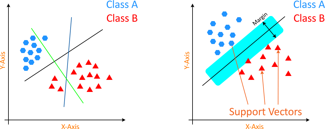
Support Vector Machines is commonly used for classification problems and it yields a better result than both regression and decision trees. It generates an ace hyperplane in an iterative manner, which is used to minimize an error. The hyperplane is that plane that separates different class elements. Look at the image below to get a basic idea of what SVM does.

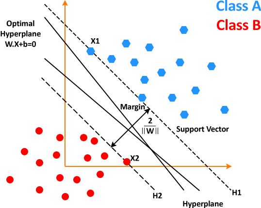
Working of SVM

Case 1: When data points are linear and separable(LInear SVM)

Begins with generating hyperplanes that sort out the classes in the best possible way.

Then selecting the right hyperplane with best sorting i.e maximum segregation from either nearest data point. The two images are shown below to give a  basic idea.

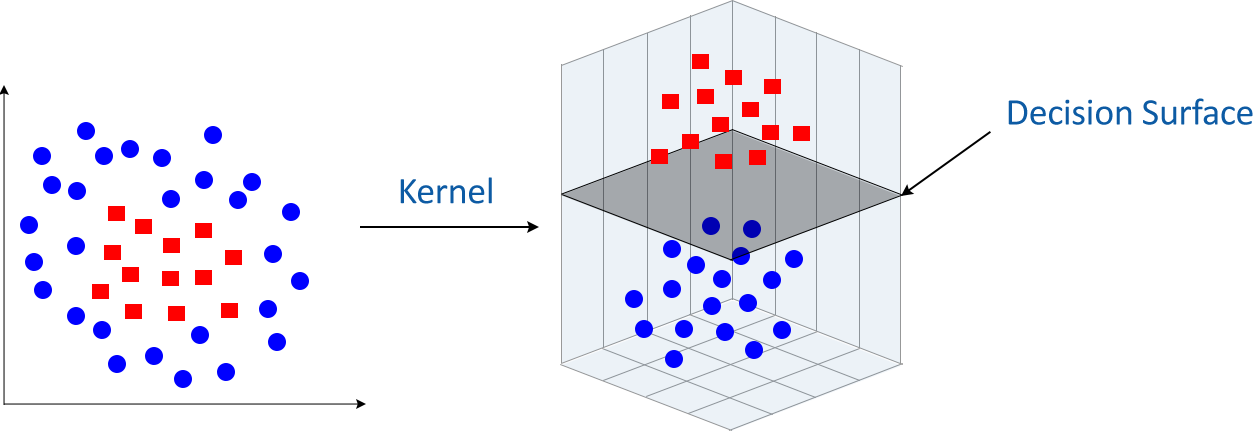
Case 2: When data points are non-linear and  inseparable(Kernel SVM)

In this case, we can't use linear hyperplanes as the data points are inseparable, unlike the previous case where data points were separable.

Now, in such conditions, SVM uses kernel trick to transform input space to a higher-dimensional space.

After the implementation of the kernel trick, these data points can be easily sorted out using linear separation. The kernel trick helps in building a more accurate classifier.

Python implementation

#import required libraries
from sklearn import datasets 
from sklearn.datasets import load_iris
from sklearn.svm import SVC

#here we will use Iris dataset too
X,y = load_iris(return_X_y =True)

#Create Model
svc = SVC(C=0.5, random_state=42)

#Feed data to model
svc.fit(X, y)

#Check training score
svc.score(X,y)

Output:

K-Nearest Neighbors(KNN)

It is one of the best, popular, and strong classifying algorithms. Here, K represents the number of nearest neighbours. It is the core deciding factor and K is generally an odd number to have a tiebreaker.

Basic Idea:  Suppose L1 is the point whose output/label we have to predict. We will start by finding K nearest points to L1 and then classify the L1 point by the majority vote of its K neighbors. Each object votes for their class and the class with the most votes is taken as a prediction. For finding nearest points we find the distance between these points using distance measurements such as Euclidean distance, Hamming distance, or Manhattan distance.

Suppose we have to classify a new unknown point either as an element Class A or Class B as shown below.

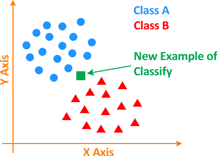
So, the question is how do we proceed?

There are 2 steps involved in classifying these unknown points which are:

1) Calculate the distance between the unknown point and the other points.

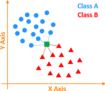
2) Find the K number of closest neighbours to the unknown point and vote for labels. In the image below, the orange circular region/boundary has the K number of closest neighbours.

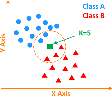
Here, K = 5; as 2 points are from Class A and 3 points from Class B. As a result of which unknown point will be classified as a Class B element.

Now, the next big question is how to select the value of K or what should be the appropriate number of nearest neighbours?

Suppose we set K = 1, in such a case our prediction will become shaky. Imagine an unknown data point to be surrounded by Class A data points but having one Class B data point nearest to it, so just because K is equal to 1 will lead to a wrong prediction. On the other hand, as we start increasing the value of K our model's prediction will improve as there will be more neighbours to classify that point but there will come a stage when our model's prediction will start to go downhill, at that point we know we have pushed the value of K too far. In short, there is no specific value of K to attain the best prediction, we have to try different values till we find the optimal value.

Python Implementation:

#import required libraries
from sklearn import datasets 
from sklearn.datasets import load_iris
from sklearn.neighbors import KNeighborsClassifier

#here we will use Iris dataset too
X,y = load_iris(return_X_y =True)

#Create Model
knn = KNeighborsClassifier(n_neighbors=7)

#Feed data to model
knn.fit(X, y)

#Check training score
knn.score(X,y)

Output:

Naive Bayes Classification

( I will encourage you to study about Bayes theorem before starting this section)

This algorithm uses the Bayes theorem of probability for the prediction of an unknown class.

Bayes theorem formula(image):  

where,

• P(A|B) is the posterior probability of class (A, target) given predictor (B, attributes).

• P(A) is the prior probability A; probability of the hypothesis being true.

• P(B|A) is the likelihood which is the probability of predictor given class.

• P(B) is the prior probability of D; probability of data.

And the term Naive means that the algorithm considers the effect of a particular feature in a class is independent of other features. Even if these features are interdependent, they are still considered independent. Such as if the banana is identified based on color, shape, and taste, then yellow, curved, and sweet fruit is recognized as a banana. Hence each feature individually contributes to identifying that it is a banana without depending on each other.

It is a time-saving, accurate and reliable algorithm.

Working of Naive Bayes

Step 1: Conversion of the data set into a frequency table.

Step 2: Creation of Likelihood table by finding the probabilities.

Step 3: Now use the Naive Bayesian equation for calculating the posterior probability for each class. The class with the highest posterior probability is the outcome of the prediction.

There is 3 type of Naive Bayes model scikit-learn provides:

1. Gaussian naïve Bayes: It is a form of Naive Bayes, it assumes that features follow a Gaussian normal distribution and is used for classification problems.

2. Multinomial naïve Bayes: It considers a feature vector where a given entity represents the number of times it appears i.e. frequency. It is mostly used in Natural Language Processing.

3. Bernoulli naïve Bayes: It is a binary algorithm used when the feature is present or not.

Python Implementation:

#import required libraries
from sklearn import datasets 
from sklearn.datasets import load_iris
from sklearn.naive_bayes import GaussianNB

#here we will use Iris dataset too
X,y = load_iris(return_X_y =True)

#Create Model
gnb = GaussianNB()

#Feed data to model
gnb.fit(X, y)

#Check training score
gnb.score(X,y)

Output:

Decision Tree

This algorithm also belongs to the family of supervised learning algorithms. The decision tree is mostly used in classification problems. It works for both categorical and continuous input and output variables. In this technique, we split the sample into two or more homogeneous sets based on the most significant input variables.

Below is an image that describes the structure and working of the decision tree.

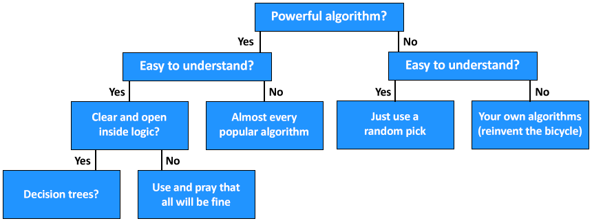
Working of the Decision Tree Algorithm 

Step1: Initiate the tree with the root node, here the Powerful algorithm? is the root node.

Step2: Using the Attribute Selection measure find the best attribute. example: Gini Index, Chi-Square, Information Gain, and Reduction in Variance.

Step3: Divide the root into subsets that hold possible values for the best attributes.

Step4: Generate the decision tree node, which contains the best attribute.

Step5: Recursively make new decision trees using the subsets of the dataset created in step -3. Continue this process until a stage is reached where you cannot further classify the nodes and called the final node as a leaf node.

Python Implementation:

#import required libraries
from sklearn import datasets 
from sklearn.datasets import load_iris
from sklearn.tree import DecisionTreeClassifier

#here we will use Iris dataset too
X,y = load_iris(return_X_y =True)

#Create Model
classifier = DecisiontreeClassifier(criterion='entropy', random_state=3)

#Feed data to model
classifier.fit(X, y)

#Check training score
classifier.score(X,y)

Output:

When to pick which algorithm?

Implementing the right algorithm in the right scenario is also an important task. Below is a decision process flowchart that shows when to pick which algorithm.

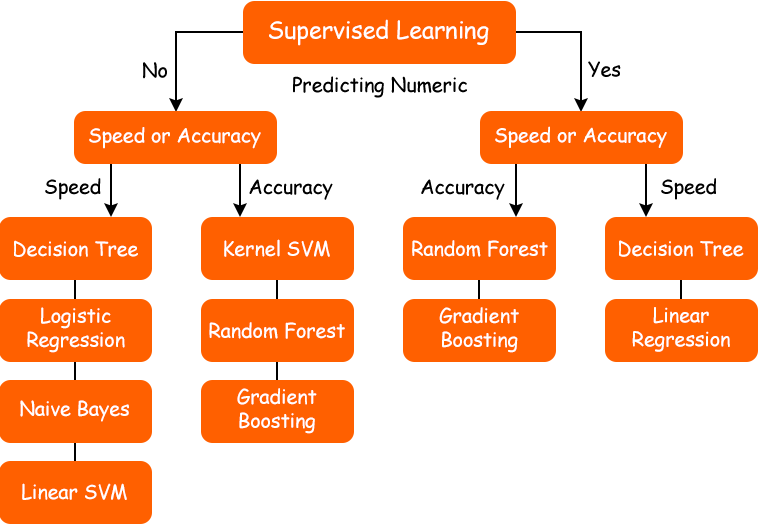
Suggestion: 

I encourage you all to read scikit-learn documentation. Also, study these algorithms and techniques: Gradient descent and cost/loss function, boosting(XGBoost, Gradient Boosting), bagging(Random Forest), and regularization to acquire more knowledge of supervised learning algorithms.

Conclusion:

This article learned about the common supervised learning algorithms and how to implement them using Python. These are not the only supervised learning algorithms known to us but they are fundamental for other advance supervised learning algorithms. The other important thing is that no algorithm is best or worst, algorithm selection completely depends upon the problem we have to deal with and the goal we have to achieve(accuracy score). Say, for regression problem linear regression may be applied for good results but for classification, it is not. 

I hope, you got an idea of supervised learning algorithms and their implementation. Still, if you have any questions leave your comment and I will be there to help you. 

Also Read Blogs On

• What is Metasploit Framework | What is Penetration Testing | How to use Metasploit
• How to Install Metasploit on Windows and Linux | [Step by Step Guide]
• What is Graph in Data Structures? | Techofide
• How To Install Arch Linux [Installation Guide] 2023 | Techofide
• Boot Menu Option Keys For All Computers and Laptops Updated List 2021 | Techofide